11. Calibration tool
Félix-Antoine Fortin, François-Michel De Rainville, Marc-André Gardner, Marc Parizeau and Christian Gagné, “DEAP: Evolutionary Algorithms Made Easy”, Journal of Machine Learning Research, vol. 13, pp. 2171-2175
Calibration method
Calibration is using an evolutionary computation framework in Python called DEAP (Fortin et al., 2012). We used the implemented evolutionary algorithm NSGA-II (Deb et al., 2002) for single objective optimization. As objective function we used the modified version of the Kling-Gupta Efficiency (Kling et al., 2012), 2012), with r as the correlation coefficient between simulated and observed discharge (dimensionless), β as the bias ratio (dimensionless) and γ as the variability ratio.

 and
and 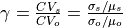
Where CV is the coefficient of variation, μ is the mean streamflow [m3 s−1] and σ is the standard deviation of the streamflow [m3 s−1]. KGE’, r, β and γ have their optimum at unity. The KGE’ measures the Euclidean distance from the ideal point (unity) of the Pareto front and is therefore able to provide an optimal solution which is simultaneously good for bias, flow variability, and correlation. For a discussion of the KGE objective function and its advantages over the often used Nash–Sutcliffe Efficiency (NSE) or the related mean squared error see (Gupta et al., 2009). The calibration uses general a population size (µ) of 256, a recombination pool size (λ) of 32.The number of generations was set to 30, which we found was sufficient to achieve convergence for stations
Further ideas for calibration
Regionalization see (Samaniego et al. 2017) and (Beck et al. 2016)
Using Budyko see (Greve et al. 2016)
Suggested Calibration parameters
Calibration tool structure
calibration
│-  readme.txt
│-  readme.txt
│
└--observed_data
│   └- lobith2006.cvs, ...
│
└--templates
│   └-- runpy.bat, runpy.sh
│   └-- settings.ini
How it works
The calibration tool builds up a single-objective obtimization framework using the Python libray DEAP For each run it triggers the run of the hydrological model:
using a template of the settings file
replacing the output folder in this template file
replace placeholders with the values of calibration parameters, the limit of the parameter range is given in the file: ParamRanges.csv
After each run the model run is compared to observed values (e.g. observed_data/lobith2006.csv)
After the calibration, statistics and the best run is printed output
What is needed
runpy.bat: the path to cwatm.py have to be set correctly (for linux a .sh file has to be created)
The actual version of a cwatm settings file has to modified:
replacing the output folder with the placeholder: %run_rand_id
28#-------------------------------------------------------
29# CALIBARTION PARAMETERS
30#-------------------------------------------------------
31[CALIBRATION]
32
33# These are parameter which are used for calibration
34# could be any parameter, but for an easier overview, tehey are collected here
35# in the calibration template a placeholder (e.g. %arnoBeta) instead of value
36
37OUT_Dir = %run_rand_id
putting the output variables in e.g. OUT_TSS_Daily = discharge or monthly average discharge OUT_TSS_MonthAvg = discharge
38OUT_TSS_Daily = discharge
39OUT_TSS_MonthAvg = discharge
delete all the output variables in the template (mostly at the end of the file)
replacing calibration parameter values with a placeholder: e.g. %SnowMelt
42# Snow  SnowMeltCoef = 0.004
43SnowMeltCoef = %SnowMelt
44# Cropf factor correction
45crop_correct =  %crop
46#Soil
47soildepth_factor = %soildepthF
48#Soil preferentialFlowConstant = 4.0, arnoBeta_factor = 1.0
49preferentialFlowConstant = %pref
50arnoBeta_add = %arnoB
51# interflow part of recharge factor = 1.0
52factor_interflow = %interF
53# groundwater recessionCoeff_factor = 1.0
54recessionCoeff_factor = %reces
55# runoff concentration factor runoffConc_factor = 1.0
56runoffConc_factor = %runoff
57#Routing manningsN factor [0.1 - 10.0] default  1.0
58manningsN = %CCM
59# reservoir  normal storage limit (fraction of total storage, [-]) [0.15 - 0.85] default 0.5
60normalStorageLimit = %normalStorageLimit
61# lake parameter - factor to alpha: parameter of of channel width and weir coefficient  [0.33 - 3.] dafault 1.
62lakeAFactor = %lakeAFactor
63# lake wind factor - factor to evaporation from lake [0.8 - 2.] dafault 1.
64lakeEvaFactor = %lakeEvaFactor
ParameterName,MinValue,MaxValue
SnowMelt,0.001,0.007
crop,0.8,3.0
soildepthF, 0.8,1.8
pref,0.5,8
arnoB,0.01,1.0
interF, 0.33,3.0
reces,0.1,10
runoff,0.1,5
CCM,0.1,10.0
normalStorageLimit,0.15,0.85
lakeAFactor,0.333,3.0
lakeEvaFactor,0.5,3.0
No,1,100
 1#-------------------------------------------------------
 2[TIME-RELATED_CONSTANTS]
 3#-------------------------------------------------------
 4
 5# StepStart has to be a date e.g. 01/06/1990
 6# SpinUp or StepEnd either date or numbers
 7# SpinUp: from this date output is generated (up to this day: warm up)
 8
 9StepStart = 1/1/1990
10SpinUp = 1/1/1995
11StepEnd =  31/12/2010
[DEFAULT]
Root = /c/watmodel/CWATM
RootPC = C:/watmodel/CWATM
Rootbasin = calibration_rhine

ForcingStart = 1/1/2000
ForcingEnd = 31/12/2010
timeperiod = daily

[ObservedData]
Qtss = observed_data/lobith.csv
Column = lobith
Header = River: Rhine  station: Lobith

[Validate]
Qtss = observed_data/lobith_val.csv
ValStart = 1/1/1990
ValEnd = 31/12/1999


[Path]
Templates = templates
SubCatchmentPath = catchments
ParamRanges = ParamRanges.csv

[Templates]
ModelSettings = settings.ini
RunModel = runpy.sh

[Option]
firstrun = False
para_first = [0.0022, 1.72, 1.24, 7.07, 0.55, 1.92, 2.81, 0.74,1.34,0.35,2.04,1.0, 1.]
# Snowmelt, crop KC, soil depth,pref. flow, arno beta, interflow factor, groundwater recession,
# runoff conc., routing, manning factor, normalStorageLimit, lakeAFactor,lakeEvaFactor,No of run
bestrun = True

[DEAP]
maximize = True
use_multiprocessing = 1
ngen = 30
mu = 256
lambda_ = 32
Recommendations
146[INITITIAL CONDITIONS]
147#-------------------------------------------------------
148
149# for a warm start initial variables a loaded
150# e.g for a start on 01/01/2010 load variable from 31/12/2009
151load_initial = False
152initLoad = $(FILE_PATHS:PathRoot)/init/Rhine_19891231.nc
153
154# saving variables from this run, to initiate a warm start next run
155# StepInit = saving date, can be more than one: 10/01/1973 20/01/1973
156save_initial = False
157initSave = $(FILE_PATHS:PathRoot)/init/Rhine
158StepInit = 31/12/1989 31/12/2010
References
Beck, H. E., A. I. J. M. van Dijk, A. de Roo, D. G. Miralles, T. R. McVicar, J. Schellekens and L. A. Bruijnzeel (2016). “Global-scale regionalization of hydrologic model parameters.” Water Resources Research 52(5): 3599-3622.
Deb, K., A. Pratap, S. Agarwal and T. Meyarivan (2002). “A fast and elitist multiobjective genetic algorithm: NSGA-II.” IEEE Transactions on Evolutionary Computation 6(2): 182-197.
Fortin, F. A., F. M. De Rainville, M. A. Gardner, M. Parizeau and C. Gagńe (2012). “DEAP: Evolutionary algorithms made easy.” Journal of Machine Learning Research 13: 2171-2175.
Greve, P., L. Gudmundsson, B. Orlowsky and S. I. Seneviratne (2016). “A two-parameter Budyko function to represent conditions under which evapotranspiration exceeds precipitation.” Hydrology and Earth System Sciences 20(6): 2195-2205.
Gupta, H. V., H. Kling, K. K. Yilmaz and G. F. Martinez (2009). “Decomposition of the mean squared error and NSE performance criteria: Implications for improving hydrological modelling.” Journal of Hydrology 377(1-2): 80-91.
Kling, H., M. Fuchs and M. Paulin (2012). “Runoff conditions in the upper Danube basin under an ensemble of climate change scenarios.” Journal of Hydrology 424-425: 264-277.
Samaniego, L., R. Kumar, S. Thober, O. Rakovec, M. Zink, N. Wanders, S. Eisner, H. Müller Schmied, E. Sutanudjaja, K. Warrach-Sagi and S. Attinger (2017). “Toward seamless hydrologic predictions across spatial scales.” Hydrology and Earth System Sciences 21(9): 4323-4346.