Calibration

Contents

• Calibration

  • Calibration method

  • Suggested Calibration parameters

  • Calibration tool structure

  • How it works

  • What is needed

  • Recommendations

  • Running calibration

  • Run runCalibration.bat

  • For testing

  • Running it on your computer

  • Preparation for another catchment

    • Preparing the observed dataset – discharge

  • Creating an initial netcdf file for warm start

  • Cutting out a catchment as mask map

  • Calibration of a downstream catchment

    • Cutting the mask map

    • Detecting the downstream point

    • Run the best calibration scenario upstream

    • Create an inflow file from the long timeseries of outlet(s)

    • Create a downstream calibration settings (directories, templates etc.)

    • Change the settings file

  • Joining best sub-basin results to calibration maps

  • References

Calibration tool for hydrological models

in ../CWatM/calibration

using a distributed evolutionary algorithms in python: DEAP library

http://deap.readthedocs.io/en/master/

https://github.com/DEAP/deap/blob/master/README.md

Félix-Antoine Fortin, François-Michel De Rainville, Marc-André Gardner, Marc Parizeau and Christian Gagné, “DEAP: Evolutionary Algorithms Made Easy”, Journal of Machine Learning Research, vol. 13, pp. 2171-2175

Note

You can install it with: Pip install deap

The calibration tool was created by Hylke Beck 2014 (JRC, Princeton) hylkeb@princeton.edu

Thanks Hylke for making it available for use and modification

Modified by Peter Burek

The submodule Hydrostats was created 2011 by:

Sat Kumar Tomer (modified by Hylke Beck)

Please see his book Python in Hydrology

Calibration method

Calibration is using an evolutionary computation framework in Python called DEAP (Fortin et al., 2012). We used the implemented evolutionary algorithm NSGA-II (Deb et al., 2002) for single objective optimization. As objective function we used the modified version of the Kling-Gupta Efficiency (Kling et al., 2012), 2012), with r as the correlation coefficient between simulated and observed discharge (dimensionless), β as the bias ratio (dimensionless) and γ as the variability ratio.

where: and

Where CV is the coefficient of variation, μ is the mean streamflow [m3 s−1] and σ is the standard deviation of the streamflow [m3 s−1]. KGE’, r, β and γ have their optimum at unity. The KGE’ measures the Euclidean distance from the ideal point (unity) of the Pareto front and is therefore able to provide an optimal solution which is simultaneously good for bias, flow variability, and correlation. For a discussion of the KGE objective function and its advantages over the often used Nash–Sutcliffe Efficiency (NSE) or the related mean squared error see (Gupta et al., 2009). The calibration uses general a population size (µ) of 256, a recombination pool size (λ) of 32.The number of generations was set to 30, which we found was sufficient to achieve convergence for stations

Suggested Calibration parameters

Snow

1. Snowmelt coefficient in [m/C deg/day] as a degree-day factor

Evapotranspiration

2. Crop factor as an adjustment to crop evapotranspiration

Soil

3. Soil depth factor: a factor for the overall soil depth of soil layer 1 and 2

4. Preferential bypass flow: empirical shape parameter of the preferential flow relation

5. Infiltration capacity parameter: empirical shape parameter b of the ARNO model

Groundwater

6. Interflow factor: factor to adjust the amount which percolates from interflow to groundwater

7. Recession coefficient factor: factor to adjust the base flow recession constant (the contribution from groundwater to baseflow)

Routing

8. Runoff concentration factor: a factor for the concentration time of run-off in each grid-cell

9. Channel Manning’s n factor: a factor roughness in channel routing

10. Channel, lake and river evaporation factor: factor to adjust open water evaporation

Reservoir & lakes

11. Normal storage limit: the fraction of storage capacity used as normal storage limit

12. Lake A factor : factor to channel width and weir coefficient as a part of the Poleni weir equation

Calibration tool structure

calibration
│-  readme.txt
│-  readme.txt
│
└--observed_data
│   └- lobith2006.cvs, ...
│
└--templates
│   └-- runpy.bat, runpy.sh
│   └-- settings.ini

How it works

The calibration tool builds up a single-objective obtimization framework using the Python libray DEAP For each run it triggers the run of the hydrological model:

• using a template of the settings file

• replacing the output folder in this template file

• replace placeholders with the values of calibration parameters, the limit of the parameter range is given in the file: ParamRanges.csv

After each run the model run is compared to observed values (e.g. observed_data/lobith2006.csv)

After the calibration, statistics and the best run is printed output

What is needed

1. The template files in ../templates have to be adjusted

• runpy.bat: the path to cwatm.py have to be set correctly (for linux a .sh file has to be created)

• The actual version of a cwatm settings file has to modified:

• replacing the output folder with the placeholder: %run_rand_id

#-------------------------------------------------------
# CALIBARTION PARAMETERS
#-------------------------------------------------------
[CALIBRATION]

# These are parameter which are used for calibration
# could be any parameter, but for an easier overview, tehey are collected here
# in the calibration template a placeholder (e.g. %arnoBeta) instead of value

OUT_Dir = %run_rand_id

• putting the output variables in e.g. OUT_TSS_Daily = discharge or monthly average discharge OUT_TSS_MonthAvg = discharge

OUT_TSS_Daily = discharge
OUT_TSS_MonthAvg = discharge

• delete all the output variables in the template (mostly at the end of the file)

• replacing calibration parameter values with a placeholder: e.g. %SnowMelt

# Snow  SnowMeltCoef = 0.004
SnowMeltCoef = %SnowMelt
# Cropf factor correction
crop_correct =  %crop
#Soil
soildepth_factor = %soildepthF
#Soil preferentialFlowConstant = 4.0, arnoBeta_factor = 1.0
preferentialFlowConstant = %pref
arnoBeta_add = %arnoB
# interflow part of recharge factor = 1.0
factor_interflow = %interF
# groundwater recessionCoeff_factor = 1.0
recessionCoeff_factor = %reces
# runoff concentration factor runoffConc_factor = 1.0
runoffConc_factor = %runoff
#Routing manningsN factor [0.1 - 10.0] default  1.0
manningsN = %CCM
# reservoir  normal storage limit (fraction of total storage, [-]) [0.15 - 0.85] default 0.5
normalStorageLimit = %normalStorageLimit
# lake parameter - factor to alpha: parameter of of channel width and weir coefficient  [0.33 - 3.] dafault 1.
lakeAFactor = %lakeAFactor
# lake wind factor - factor to evaporation from lake [0.8 - 2.] dafault 1.
lakeEvaFactor = %lakeEvaFactor

2. the range of parameter space has to be defined in ParamRanges.csv

ParameterName,MinValue,MaxValue
SnowMelt,0.001,0.007
crop,0.8,3.0
soildepthF, 0.8,1.8
pref,0.5,8
arnoB,0.01,1.0
interF, 0.33,3.0
reces,0.1,10
runoff,0.1,5
CCM,0.1,10.0
normalStorageLimit,0.15,0.85
lakeAFactor,0.333,3.0
lakeEvaFactor,0.5,3.0
No,1,100

3. The observed discharge has to be provided in an .cvs file e.g. observed_data/lobith2006.csv

In the template settings the date has to be set, so that the period of observed discharge is between SpinUp and StepEnd

#-------------------------------------------------------
[TIME-RELATED_CONSTANTS]
#-------------------------------------------------------

# StepStart has to be a date e.g. 01/06/1990
# SpinUp or StepEnd either date or numbers 
# SpinUp: from this date output is generated (up to this day: warm up)

StepStart = 1/1/1990
SpinUp = 1/1/1995
StepEnd =  31/12/2010

4. And empty ../catchments directory needs to be created

5. A few option in the settings.txt have to be adjusted (how many runs?, a first run with standard parameters? etc)

[DEFAULT]
Root = /c/watmodel/CWATM
RootPC = C:/watmodel/CWATM
Rootbasin = calibration_rhine

ForcingStart = 1/1/2000
ForcingEnd = 31/12/2010
timeperiod = daily

[ObservedData]
Qtss = observed_data/lobith.csv
Column = lobith
Header = River: Rhine  station: Lobith

[Validate]
Qtss = observed_data/lobith_val.csv
ValStart = 1/1/1990
ValEnd = 31/12/1999


[Path]
Templates = templates
SubCatchmentPath = catchments
ParamRanges = ParamRanges.csv

[Templates]
ModelSettings = settings.ini
RunModel = runpy.sh

[Option]
firstrun = False
para_first = [0.0022, 1.72, 1.24, 7.07, 0.55, 1.92, 2.81, 0.74,1.34,0.35,2.04,1.0, 1.]
# Snowmelt, crop KC, soil depth,pref. flow, arno beta, interflow factor, groundwater recession,
# runoff conc., routing, manning factor, normalStorageLimit, lakeAFactor,lakeEvaFactor,No of run
bestrun = True

[DEAP]
maximize = True
use_multiprocessing = 1
ngen = 30
mu = 256
lambda_ = 32

6. run python calibration_single.py settings.txt

Recommendations

1. Run the model first to store the pot. evaporation results

Afterwards use the stored evaporation to run the calibration

calc_evaporation = False

2. Run the model and store the last day to be used as initial condition for the calibration runs

Best is to use a long term run for this.

[INITITIAL CONDITIONS]
#-------------------------------------------------------

# for a warm start initial variables a loaded
# e.g for a start on 01/01/2010 load variable from 31/12/2009
load_initial = False
initLoad = $(FILE_PATHS:PathRoot)/init/Rhine_19891231.nc

# saving variables from this run, to initiate a warm start next run
# StepInit = saving date, can be more than one: 10/01/1973 20/01/1973
save_initial = False
initSave = $(FILE_PATHS:PathRoot)/init/Rhine
StepInit = 31/12/1989 31/12/2010

load_initial = False

save_initial = True

During calibration use:

load_initial = True

save_initial = False

3. Use a long SpinUp time (> 5 years to give groundwater enough time)

Running calibration

1. Look into the settings file of the calibration folder.

2. look into runCalibration.bat. If python is in your computer path everything should be ok, otherwise put in the path to python

3. look into templates/runpy.bat. Put the path to python in if necessary

4. look into templates/settings.ini. Put the pathes in a right way that it fits to your computer:

   [FILE_PATHS]
   #-------------------------------------------------------
   PathRoot = P:/watmodel/CWatM/calibration_tutorial
   PathOut = $(PathRoot)/output
   PathMaps = $(PathRoot)/CWatM_data/cwatm_input
   PathMeteo = $(PathRoot)/climate
   

5. in observed_data/yukon2001.cvs you find the observed data:

   - make sure the name in the header is the same as in [ObservedData] Column
   - make sure that there are enough data in (from ForcingStart to ForcingEnd)
   

6. make sure the folder catchments is empty! Before each try this folder has to be empty

Run runCalibration.bat

1. go for testing (see below)

2. go for testing again (see below)

3. Change use_multiprocessing =1 in settings.txt

4. Run runCalibration.bat and after some time something should appear on your window

For testing

• Change use_multiprocessing = 0 in settings.txt

• Delete catchments but keep the empty folder

• Run runCalibration.bat and wait till catchment/00_001 gets filled, then interrupt

1. Change to catchments/00_001

2. Run runpy00_001.bat

3. See what errors come up and change settings-Run00_001.ini

4. Change template/setting.ini in the same way

5. Do this again and again till no error

Running it on your computer

It will be really slow on Windows using data on the the server – next step run it on your PC

• copy the whole folder P:watmodelCWatMcalibration_tutorial to your PC (only 15 GB)

• (but maybe you have already parts of it on your computer – like the big climate input files)

• Make it work on your computer:

  Changing file paths in templates/settings.ini, setting.txt
  Changing the path for python in runCalibration.bat and templates/runpy.bat
  

Preparation for another catchment

Preparing the observed dataset – discharge

Calibration works by comparing simulated discharge with observed discharge using an objective function: Here we use the Kling-Gupta Efficiency but we can also use Nash-Sutcliffe Efficiency . Please find some more information on the objective function an on the evolutionary computation framework used for calibration on: https://cwatm.github.io/calibration.html

• The observed values can be stored as daily values or monthly values

• The observed values should be at least cover 5 years (best is 10-15 years)

• The observed discharge has to be stored as textfile in:

  ./observed_data/nameofstation.cvs
  And has to look like this:
  date,yukon_pilot_station
  2001-04-01,1302.6
  2001-04-02,1302.6
  2001-04-03,1302.6
  2001-04-04,1302.6
  …
  …
  2013-12-31,2647.6
  

• Or:

  date ,zhutuo
  2002-01-01,3229.0
  2002-02-01,2979.2
  2002-03-01,3229.0
  

Format:

• Date format like this year-month-day [yyyy-mm-dd]

• Separated by a comma

• Discharge in [m3/s]

• If a value is missing that is not a problem (as long as the time series is long enough):

  it should like this: (no value after the comma)
  2002-01-12,
  

• For each day (or month) a line

Settings.txt

In the settings file the lines:

[ObservedData]
Qtss = observed_data/zhutuo_2002month.csv
Column = zhutuo
Header = River: Yangtze  station: Zhutuo

Should correspondent to the name and header in the observed discharge.cvs

The lines:

ForcingStart = 1/1/2002
ForcingEnd = 31/12/2013

Should correspondent to the amount of lines in the observed discharge.cvs

Creating an initial netcdf file for warm start

It is best to have a long warm up phase especially for groundwater: See also: https://cwatm.github.io/setup.html#initialisation

You can run CWatM for a couple of years (20 years or more) and store the last days storage values in a file. This file can be read in to enable a ‘warm” start

• change use_multiprocessing = 0 in settings.txt

• Delete catchments but keep the empty folder

• Run runCalibration.bat and wait till catchment/00_001 gets filled, then interrupt

• Change to catchments/00_001

Open the settings-Run_001.init

• Change load_initial = True to load_initial = False

• save_initial = True

• initSave = $(FILE_PATHS:PathRoot)/CWatM_init/testx

• StepInit = 31/01/1996 (change it to a date 1 month after your StepStart)

• Run runpy00_001.bat

There should be a file ./CWatM_init/testx_19960131.nc

• Change to: load_initial = True

• initLoad = $(FILE_PATHS:PathRoot)/CWatM_init/testx_19960131.nc

• Run runpy00_001.bat

If it work then it used the initial file you generate before (that was just a test)

Now change to:

• StepStart = 1/1/1961

• StepEnd = 31/12/2013

• load_initial = False

• save_initial = True

• initSave = $(FILE_PATHS:PathRoot)/CWatM_init/station_name

• StepInit = 31/12/2013

• Run runpy00_001.bat

This should have generated a file ./CWatM_init/station_name_20131231.nc

And again:

• StepStart = 1/1/1961 (some 20 years or longer)

• StepEnd = 31/12/1995 (a day before your normal running day)

• load_initial = True

• initLoad = $(FILE_PATHS:PathRoot)/CWatM_init/station_name_20131231.nc

• save_initial = True

• initSave = $(FILE_PATHS:PathRoot)/CWatM_init/station_name

• StepInit = 31/12/1995 (a day before your running day)

• Run runpy00_001.bat

This should have generated a file ./CWatM_init/station_name_19951231.nc

And last part:

• Change StepStart and StepEnd back to original values

• load_initial = True

• initLoad = $(FILE_PATHS:PathRoot)/CWatM_init/station_name_19951231.nc

• save_initial = False

• Run runpy00_001.bat

If it works, do the same in the ./template/settings.ini

Note

You have now a “warm” start for every calibration run

Cutting out a catchment as mask map

See the .doc file in P:watmodelCWatMcalibration_tutorialcalibrationtoolscut_catchmentFor a description:

Requirements: PCRASTER:

We do no need the python version, I think downloading, extracting and setting of the paths in P:watmodelCWatMcalibration_tutorialcalibrationtoolscut_catchmentcatchconfig_win.ini Creating the 2 potential evaporation files in advance

Potential evaporation is Calculated with Penman-Monteith in CWatM, but it is not part of the calibration = there is no change in pot. Evaporation. In order to make the calibration computational faster the results of pot evaporation could be stored and used every time.

For the 30min this is done already as global map set, but for the 5min these files become too big. So they have to be produced for each basin separately

Same preparation as for Creating an initial netcdf file for warm start see above There should be a folder catchments00_001 with a working run for 001.

Open the settings-Run_001.init

Change:

[Option] calc_evaporation = True
[TIME-RELATED_CONSTANTS] SpinUp = None
[EVAPORATION]
OUT_Dir = $(FILE_PATHS:PathOut)
OUT_MAP_Daily = ETRef, EWRef

Run runpy00_001.bat

There should be a file ETRef.nc and EWRef in the output directory

Rename the files e.g. ETRef.nc to ETRef_yangtze.nc, EWRef.nc to EWRef_yangtze.nc and copy it to PathMeteo (or somewhere else, you have to put the path in)

Open the settings-Run_001.init

Change:

[Option] calc_evaporation = False
[TIME-RELATED_CONSTANTS] SpinUp = -> to the time it was before
[Meteo]
daily reference evaporation (free water)
E0Maps = $(FILE_PATHS:PathMeteo)/EWRef_yangtze
daily reference evapotranspiration (crop)
ETMaps = $(FILE_PATHS:PathMeteo)/ETRef_yangtze
[EVAPORATION]
OUT_Dir = $(FILE_PATHS:PathOut)       !!! outcomment this again - important
OUT_MAP_Daily = ETRef, EWRef

Test it: Run runpy00_001.bat

And change the settings.ini in templates in the same way

Calibration of a downstream catchment

Calibration of a downstream catchment (upstream catchment is already calibrated) can be done using:

• The catchment area of the downstream catchment minus the upstream catchment

• The missing discharge from the upstream catchment is replaced by an inflow file

1. Cut the mask map, so that the upstream catchment is NOT in the mask map anymore

2. Detect the point(s) downstream of the inflow points

3. Run the best calibration scenario(s) of the upstream catchments again to produce long timeserie(s) of the outlet(s) point

4. Create an inflow file from the long timeseries of outlet(s)

5. Create a downstream calibration settings (directories, templates etc.)

Test the catchment!

6. Change the settings file of the downstream calibration so that it includes the inflow from upstream

Test it! 7. Create initial file for warm start

Cutting the mask map

Assuming you have a mask map of the whole catchment (e.g. Yangtze.map and the station points (here Zhutuo 105.75 28.75 and Yichang 111.25 30.75 1. Creating catchment for Zhutuo: catchment 105.75 28.75 ldd_yangtze.map zhu1.map 2. Creating catchment for Yichang: catchment 111.25 30.75 ldd_yangtze.map yi1.map 3. Creating Yichang without Zhutuo:

pcrcalc a2.map = cover(scalar(zhu1.map)*2,scalar(yi1.map))
pcrcalc yichang.map = boolean(if(a2.map eq 1,a2.map))

Result is a maskmap: Yichang.map

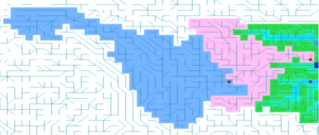
Figure 1: Upstream catchment (blue) and downstream catchment (red)

Detecting the downstream point

The inflow point of the new catchment has to be in the new mask and preferable one grid cell in flow direction below the upstream station e.g. 1 gridcell North East of Zhutuo (see purple circle in fig. 2)

The inflow point has the lon/lat 106.25 29.25

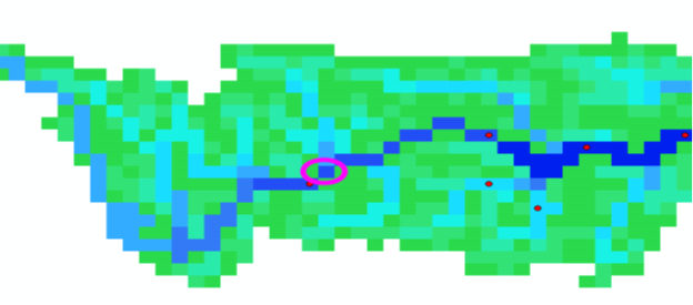
Figure 2: Downstream point

Run the best calibration scenario upstream

In order to get a long inflow timeserie for the inflow point (here: Zhutuo) you need to run the best scenario of the upstream catchment (here: 31_best)

• Change into the folder ../catchments/best

• Change settings file from:

  StepStart = 1/1/1996
  SpinUp = 1/1/2002
  StepEnd =  31/12/2013
  

• To:

  StepStart = 1/1/1990
  SpinUp = 1/1/1996
  StepEnd =  31/12/2013
  

Results is a time series from 1/1/1990 – 31/12/2013 in: discharge_daily.tss

Create an inflow file from the long timeseries of outlet(s)

• Create a folder ../inflow

• Copy the ../catchments/31_best/discharge_daily.tss to ../inflow/zhutuo.tss

Create a downstream calibration settings (directories, templates etc.)

Create downstream calibration settings as before

• Copy everything from upstream catchment (e.g. zhutuo) but not catchments

• Create empty catchments folder

• Create a observed discharge file in observed

• Change settings.txt accordingly

• Change settings.ini accordingly

Test the catchment setting!

But do not create an initial run yet!

Change the settings file

Change the settings file of the downstream calibration so that it includes the inflow from upstream Change the part of the settings.ini:

[Option]
inflow = True
[INFLOW]
#-------------------------------------------------------
# if option inflow = true
# the inflow from outside is added as inflowpoints
In_Dir = $(FILE_PATHS:PathRoot)/calibration/calibration_yichang/inflow
# nominal map with locations of (measured)inflow hydrographs [cu m / s]
InflowPoints = 106.25 29.25
InLocal = True
.
# if InflowPoints is a map, this flag is to identify if it is global (False) or local (True)
# observed or simulated input hydrographs as time series [cu m / s]
# Note: that identifiers in time series have to correspond to InflowPoints
# can be several timeseries in one file or different files e.g. main.tss mosel.tss
QInTS = zhutuo.tss

Test it!

Generate initial file for warm start Use initial file for calibration

Joining best sub-basin results to calibration maps

1. You need all runs done for all sub-basins

2. A region map

For each subbasin a unique number e.g. Zambezi basin

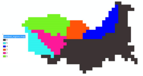
Figure 3 Sub-basin map with a unique identifier for each subbasin

3. You need a working PCRaster installation

4. The settings file settings.txt has to be changed:

   [DEFAULT]
   Root = P:/watmodel/CWatM/calibration/calibration_zambezi
   # root directory where all subbasin are in
   .
   [Catchments]
   catch = lukulu, katima, kafue, luangwa, kwando, tete
   # name of the subbasin, has to be the same as the folder name in root
   # the order has to be the same as in the region map
   .
   [region]
   regionmap = P:/watmodel/CWatM/calibration_tutorial/calibration/CreateCalibrationMaps/zambezi_regions.map
   # region map, the order has to be the same a [Catchment]
   .
   [Path]
   Templates = %(Root)s/templates
   SubCatchmentPath = %(Root)s/catchments
   ParamRanges = %(Root)s/Join/ParamRanges.csv
   .
   Result = P:/watmodel/CWatM/calibration_tutorial/calibration/CreateCalibrationMaps/results
   # here are the results
   .
   PCRHOME = C:\PCRaster\bin
   # Where is your PCraster installation?
   

5. Run python CAL_5_PARAMETER_MAPS.py

References

• Beck, H. E., A. I. J. M. van Dijk, A. de Roo, D. G. Miralles, T. R. McVicar, J. Schellekens and L. A. Bruijnzeel (2016). “Global-scale regionalization of hydrologic model parameters.” Water Resources Research 52(5): 3599-3622.

• Deb, K., A. Pratap, S. Agarwal and T. Meyarivan (2002). “A fast and elitist multiobjective genetic algorithm: NSGA-II.” IEEE Transactions on Evolutionary Computation 6(2): 182-197.

• Fortin, F. A., F. M. De Rainville, M. A. Gardner, M. Parizeau and C. Gagńe (2012). “DEAP: Evolutionary algorithms made easy.” Journal of Machine Learning Research 13: 2171-2175.

• Greve, P., L. Gudmundsson, B. Orlowsky and S. I. Seneviratne (2016). “A two-parameter Budyko function to represent conditions under which evapotranspiration exceeds precipitation.” Hydrology and Earth System Sciences 20(6): 2195-2205.

• Gupta, H. V., H. Kling, K. K. Yilmaz and G. F. Martinez (2009). “Decomposition of the mean squared error and NSE performance criteria: Implications for improving hydrological modelling.” Journal of Hydrology 377(1-2): 80-91.

• Kling, H., M. Fuchs and M. Paulin (2012). “Runoff conditions in the upper Danube basin under an ensemble of climate change scenarios.” Journal of Hydrology 424-425: 264-277.

• Samaniego, L., R. Kumar, S. Thober, O. Rakovec, M. Zink, N. Wanders, S. Eisner, H. Müller Schmied, E. Sutanudjaja, K. Warrach-Sagi and S. Attinger (2017). “Toward seamless hydrologic predictions across spatial scales.” Hydrology and Earth System Sciences 21(9): 4323-4346.