A lake is the landscape's most beautiful
and expressive feature. It is Earth's eye;
looking into which the beholder measures
the depth of his own nature
Henry David Thoreau, Walden

3. The Community Water Model

Contents

• 3. The Community Water Model

  • Model Philosophy

  • FAIR(R) software

  • Model design and processes

  • Features of the Model

  • Performance

Model Philosophy

Open source/ open data/ open community

“Open source software embodies three ideals: freedom, collaboration, and transparency within the sphere of software development. If anything, this is a methodology or even a licensing model, reflecting a philosophy whose underpinnings are deeply rooted in values about how technology is to be created, shared, and used. The principles of open source are based on the convictions that technologies must empower and not constrain, and that the greatest innovations come from joint efforts.“ (Medium.com, Diaa Atya: The Philosophy and Ethics Behind Open-Source Software - 26/10/2025)

We think users should have the freedom to use, study, share, and change our software without restriction (ok, we have restrictions: to cite use and to stick to the license). This freedom will allow users to deploy CWatM to their needs and maybe go even further than we intended, as developers. Our software has an open source code. We hope that this transparency will help us build trust. The users have the possibility to see how it all works.

Open source goes in line with IIASA`s policy: https://iiasa.ac.at/publications/open-access

Function follows form

Function follows form is the inverse design principle of Bauhaus.

For CWatM the form (the structure) is given by: - non-hydrological parts e.g. (data management, management of date/time, output functions) - hydrological functions

• hydrological processes (e.g. snow, soil, routing)

• hydrological subprocesses or alternative ways to calculate this.

Hydrological processes are split up: - initialization phase, where static, non-temporal data are read - dynamic phase, where the model runs through the time period

CWatM functions follow this form, to ensure that the code is not redundant and easy to follow.

FAIR(R) software

The FAIR principles were published in 2016 in:

Wilkinson, M., Dumontier, M., Aalbersberg, I. et al. The FAIR Guiding Principles for scientific data management and stewardship. Sci Data 3, 160018 (2016). https://doi.org/10.1038/sdata.2016.18

And used on software in: Barker, M., Chue Hong, N.P., Katz, D.S. et al. Introducing the FAIR Principles for research software. Sci Data 9, 622 (2022). https://doi.org/10.1038/s41597-022-01710-x

FAIR software refers to research software that adheres to the Findable, Accessible, Interoperable, and Reusable principles, adapted from data management to make software easier for humans and machines to discover, use, and share.

We put in another R (Reproducible) – research software should be able to produce the same results given the same environment.

Findable (F)

Software and its associated metadata must be easy to discover by humans and machines

Software is assigned a globally unique and persistent identifier, like a DOI.

- CWatM: https://doi.org/10.5281/zenodo.10044318

It is described using rich metadata, which are also FAIR and searchable.

- https://iiasa.ac.at/models-tools-data/cwatm

- https://cwatm.iiasa.ac.at/

Different versions of the software have distinct identifiers.

- Yes

Software is registered in a repository or registry to improve its visibility.

- https://github.com/iiasa/CWatM

- https://doi.org/10.5281/zenodo.10044318

Accessible (A)

In order to reuse software, the software and its metadata must be retrievable by standard protocols, free and legally usable

Software has a license:

- CWatM: GNU General public license V3. See GNU General public license.

The protocol is open, free, and universally implementable.

- The source code is open and free (according to the license) to use

Interoperable (I)

When interacting with other software it must be done by exchanging data and/or metadata through standardised protocols and application programming interfaces

Software reads, writes and exchanges data in a way that meets domain-relevant community standards.

- CWatM uses standard output formats like netcdf and .csv

Software includes qualified references to other objects.

- CWatM source code classes and functions are documented using a numpy doc format.

Reusable (R)

Software is described with a plurality of relevant attributes.

- CWatM has a documentation of the software (the webpage you are looking at)

It has a clear and accessible license, which is vital for reuse.

- CWatM: GNU General public license V3. See GNU General public license.

Software includes qualified references to other software

- Yes

The software meets community standards to ensure it can be understood, modified, or built upon

- We hope so, but our experience that the software is used and modified by others shows this.

Reproducible (R)

Model results can be reproduced with the same input data, model version, and Python environment settings. This is not stated in the FAIR principles, but over the years, we have had to put in additional effort to determine which model version and dataset were used to produce the results. To facilitate this process, we put the metainformation in the result files. The name and the date of the settingsfile and the github hash number in the header line of the timeseries results and into the global attributes of the output netcdf files.

In addition, we include the complete settings file, the names and creation dates of all input data, and the Python and library versions in each discharge output netCDF.

Note

A description how to recover the information is given in: recover or reproduce former runs

Model design and processes

The Community Water Model (CWatM) will be designed to assess water availability, water demand and environmental needs. It includes an accounting of how future water demands will evolve in response to socioeconomic change and how water availability will change in response to climate.

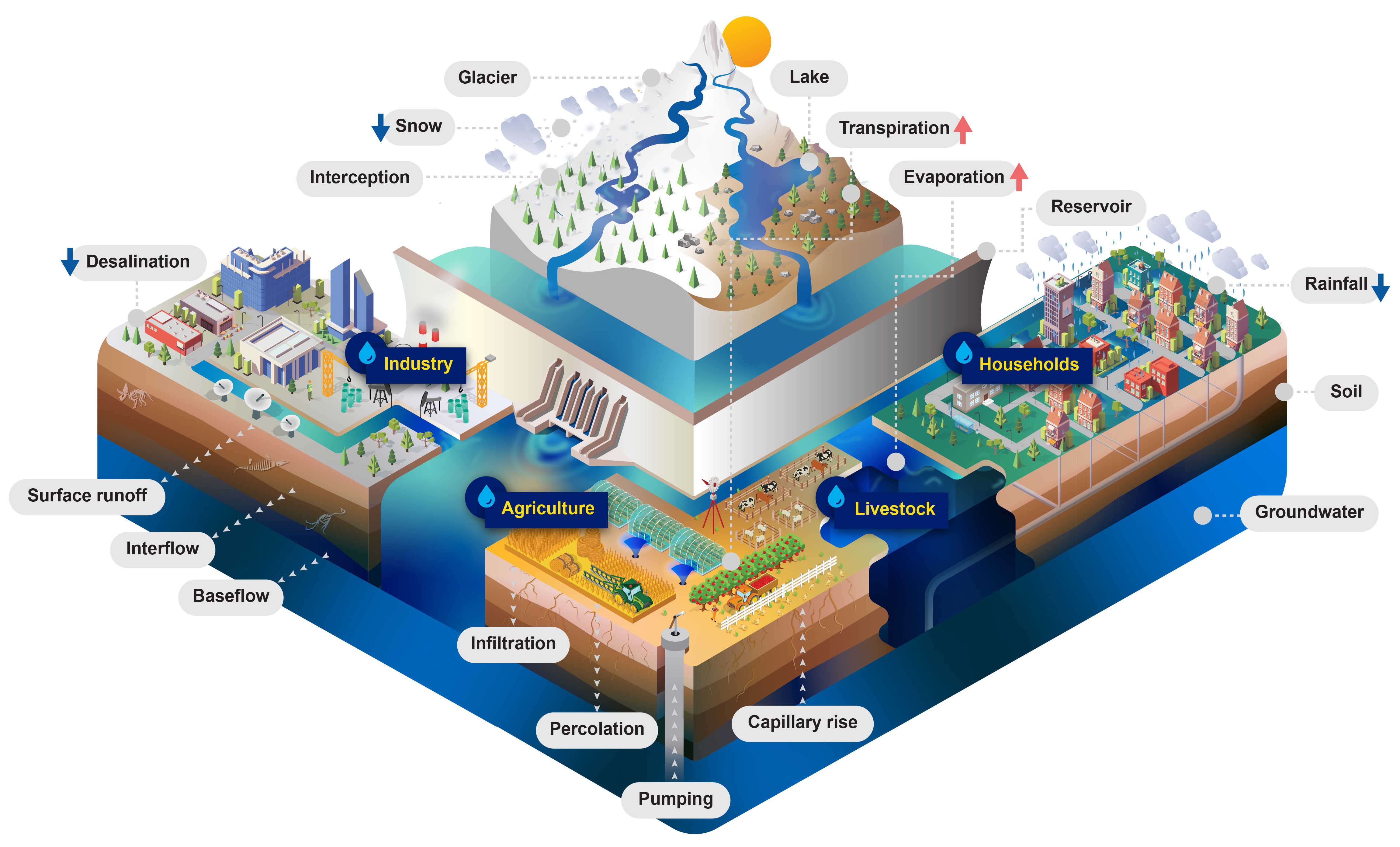
Figure 3: CWatM - Water-related processes included in the model design

Processes

Calculation of potential Evaporation

Using Penman-Montheith equations based on FAO 56

Calculation of rain, snow, and snowmelt

Using day-degree approach with up to 10 vertical layers Including snow- and glacier melt.

Land cover

using fraction of 6 different land cover types

• Forest

• Grassland

• Irrigated land

• Paddy irrigated land

• Sealed areas (urban)

• Water

Water demand

• including water demand from industry and domestic land use via precalculated monthly spatial maps

• including agricultural water use from the calculation of plant water demand and livestock water demand

• Return flows ((water withdrawn but not consumed and returned to the water circle)

Vegetation

Vegetation is taken into account in the calculation.

• Albedo

• Transpiration (including rooting depth, crop phenology, and potential evapotranspiration)

• Interception

Soil

Three soil layers for each land cover type, including processes:

• Frost interrupts soil processes

• Infiltration

• Preferential flow

• Capillary rise

• Surface runoff

• Interflow

• Percolation into groundwater

Groundwater

Groundwater storage is simulated as linear groundwater reservoir

Lakes & Reservoirs

• Lakes are simulated with weir function from Poleni for rectangular weir.

• Reservoirs are simulated as outflow function between three storage limits (conservative, normal,flood) and three outflow functions (minimum, normal, non-damaging)

Routing

Routing is calculated using the kinematic wave approach

Features of the Model

Community Model

Feature	Description
Programming Language	Python 3.x with some C++ for computational demanding processes e.g. river routing
Community driven	Open-source but lead by IIASA GitHub repository
Well documented	Documentation, automatic source code documentation
Easy handling	Use of a setting file with all necessary information for the user Complete settings file and Output meta information
Multi-platform	Python 3.x on Windows, Mac, Linux, Unix - to be used on different platforms (PC, clusters, super-computers)
Modular	Processes in subprograms, easy to adapt to the requirements of options/ solutions

Water Model

Feature	Description
Flexible	different resolution, different processes for different needs, links to other models, across sectors and across scales
Adjustable	to be tailored to the needs at IIASA i.e. collaboration with other programs/models, including solutions and option as part of the model
Multi-disciplinary	including economics, environmental needs, social science perspectives
Sensitive	Sensitive to option / solution
Fast	Global to regional modeling – a mixture between conceptional and physical modeling – as complex as necessary but not more
Comparable	Part of the ISI-MIP community

Performance

Computational run time (on a linux single node - 2400 MHz with Intel Xeon CPU E5- 2699A v4):

Daily timestep on 0.5 deg

Global: 100 years in appr. 12h = 7.2min per year

	Process	sum % runtime
1	Read Meteo Data	6.2
2	Et pot	7.6
3	Snow	8.8
4	Soil	59.4
5	Groundwater	59.5
6	Runoff conc	70.1
7	Lakes	70.4
8	Routing	95.5
9	Output	100

For the global setting, soil processes with 50% computing time is the most time consuming part, followed by routing with 25% and runoff concentration with 10%. (Reading the full global maps takes only 1/3 longer than reading a part of the global maps)

Rhine: 640 years in appr. 4.5h = 0.4min per year

	Process	sum % runtime
1	Read Meteo Data	79.4
2	Et pot	80.5
3	Snow	80.9
4	Soil	88.8
5	Groundwater	88.9
6	Runoff conc	89.6
7	Lakes	89.8
8	Routing	99.6
9	Output	100

For the Rhine basin reading input maps 79% is by far the most time consuming process, followed by routing (kinematic wave) 10% and the soil processes (8%).